For inputted lncRNAs, AnnoLnc2 will first try to map them against the latest human (hg38) and mouse (mm10) genome builds using Blat (Kent, 2002). During the mapping, AnnoLnc2 tries to associate the inputted lncRNAs with known ones by searching GENCODE gene models (v32 for human, and vM23 for mouse) based on genomic location and intron/exon structure, and matched hits will be reported as part of genomic mapping results. When a single sequence is aligned in multiple places, genome-wide best alignments are identified by standard pslSort and pslReps. In case of false-positive junction sites caused by mismatches or small indels, putative exons shorter than 20bp (as well as putative introns shorter than 40bp) are discarded. And known transcripts within upstream 5Kb and downstream 1Kb are extracted and sent to the UCSC genome browser to be presented as genomic context of the lncRNA in pre-tuned custom track.

RNAfold v2.4.14 in the ViennaRNA package (Lorenz, et al., 2011) is employed to predict secondary structures, with option “--noLP” enabled to avoid undesirable isolated base pairs. When multiple candidates available, the one with minimum free energy is kept, as being recommended by the authors of ViennaRNA package.

LncRNAs exhibit temporal-space expression with sophisticated regulations. Based on the LocExpress algorithm, AnnoLnc2 implements on-the-fly expression profiling in hundreds of samples. Specifically, AnnoLnc2 Web Server supports simultaneously expression calling in 95 human samples (52 normal tissue samples, 39 CCLE cancer cell lines as well as 4 ENCODE cell line samples) or 69 mouse samples (56 normal tissue samples and 13 ENCODE cell line samples) for any lncRNA, in nearly real time.(see here for the number of mapped reads and sample IDs).

Technically, AnnoLnc2 will compare its transcript structure identified by genomic location module with known transcripts in GENOCODE gene model using CuffCompare (version v2.2.1). If the code is “=” or “c”, the lncRNA will be considered as a "known transcript", and AnnoLnc2 will return pre-calculated expression profile of this transcript directly; otherwise it will be considered as a "novel transcript", and AnnoLnc2 will use LocExpress algorithm to estimate expression profile on-the-fly. The FPKM of two replicates of each tissue/cell line are averaged to report to users.

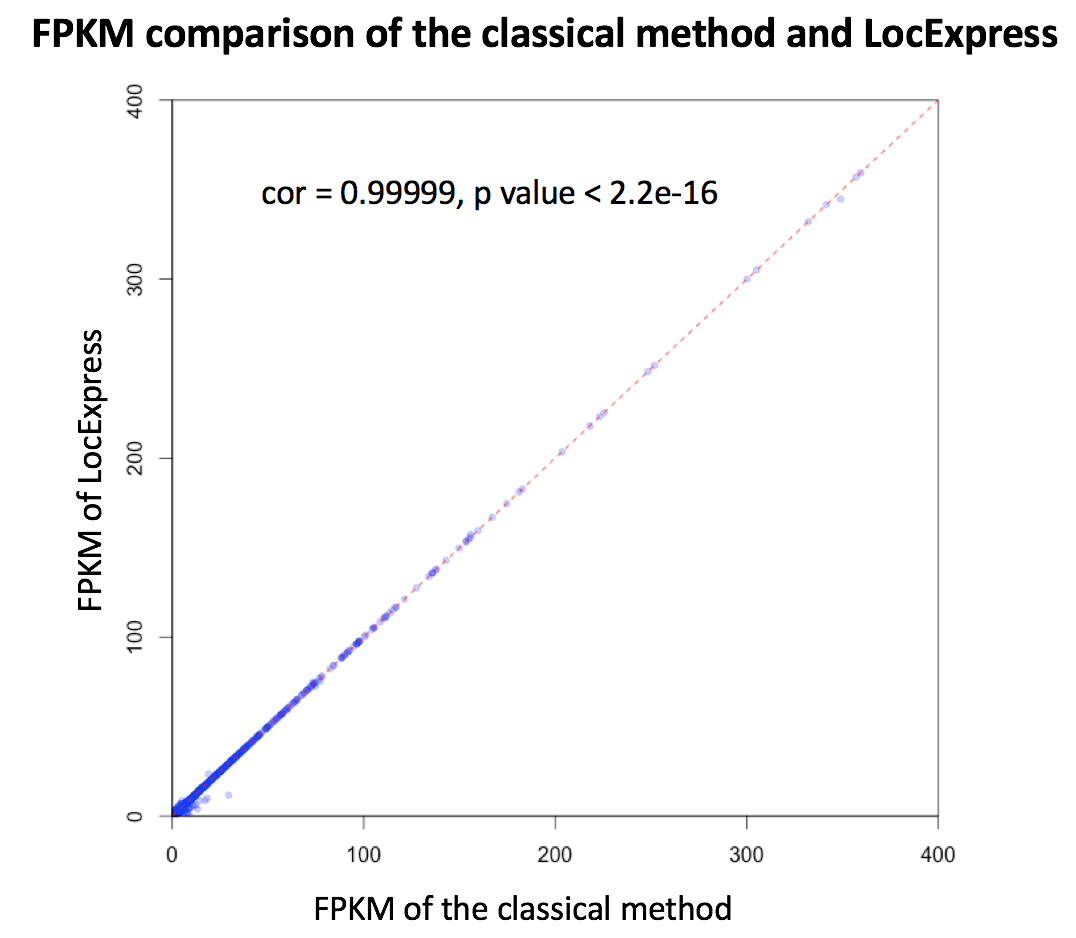
Taking advantage of the local nature of RNA-Seq, we developed a novel quantification method named LocExpress (Hou et al.) for real-time estimating expression level based on pre-mapped reads. Briefly, LocExpress will infer the Minimum Spanning Bundle (MSB) of an input transcript based on its genomic coordination as well as reads mapped in corresponding regions. Then the estimated relative abundance will be further adjusted and normalized based on original size (i.e. the total mass derived from all mapped reads) and reported in canonical FPKM unit. In our preliminary assessment, the LocExpress method usually takes less than one minute for one novel lncRNA across all samples, and the result is highly consistent with of the classical method (see the figure below).

Normal samples of human (or tissue samples of mouse) and cancer samples of human (or cell line samples of mouse) are treated separately. To avoid the duplicated GO annotation for isoforms, we firstly got expression profiles at the gene level by adding the FPKM of all transcripts of each gene in the gene model file. Then we filtered these genes as follows.

1. FPKM filter. The sum of FPKM in all samples should be not less than 1.
2. Tissue specific filter. The tissue specific score is calculated by the function “getsgene” in the R package rsgcc. If a gene has a score larger than 0.85, it’s not considered fit for the co-expression analysis.

For any submitted transcripts passed above filters, the Pearson correlation with genes is calculated. Then highly correlated genes will be reported by a “gradually decreased” criteria to remove putative false positives and retain true positives. If there are more than 10 genes with r>=0.9, we will stop here and do the GO enrichment analysis with these genes. If not, we will see whether there are 10 genes above the cutoff 0.8. This process will continue until the cutoff arrives 0.7. Negatively correlated genes are identified in a similar way. GO enrichment analysis for these correlated genes will be further conducted with the R package GOstats, and significantly enriched GO terms (adjusted p-value <= 0.01) will be reported as putative functional assignments of the input transcript.

Several recent studies have well demonstrated that, in addition to expression level, the subcellular localization of lncRNA is also under intricate regulation. As an attempt to map lncRNAs subcellular localization landscape at fine-scale, we designed and implemented a novel module to characterize lncRNAs’ cytoplasmic/nuclear localization preference empirically in ten human ENCODE cell lines. Briefly, the inputted lncRNAs will be compared with a pre-compiled localization catalog, AnnoLnc2 then returns its localization preference measured by fold change of nuclear/cytosolic expression in all ten cell lines, along with corresponding FDR-adjusted p-value.

Specifically, we downloaded raw long poly-A plus RNA sequencing data of nuclear or cytosolic fraction from GEO (GSE30567), and mapped them to reference genome (hg38) by HISAT2 (version v2.0.4). Then we used StringTie (version v1.3.0) to profile nuclear/cytosolic expression based on GENCODE annotation (v25), and discarded lowly expressed transcripts (i.e., FPKM < 0.1 in all samples). Finally, we converted FPKM to read counts with script prepDE.py from StringTie package and performed differential analysis across subcellular compartments using DESeq2 (version v1.18.1).

AnnoLnc2 integrated Transcription Factors (TFs) binding sites from GTRD database (metaclusters in version 19.10), with 91.7 million ChIP-Seq-based binding sites for 1,339 human TFs as well as 80.8 million sites for 738 mouse TFs. For each input transcript, AnnoLnc will search putative TF binding sites within upstream 5Kb and downstream 1Kb, and report all sites based on their relative position to the transcript, as “upstream transcriptional start site (TSS)”, “overlap with TSS”, “inside the lncRNA loci”, “overlap with transcriptional end site (TES)” and “downstream TES”. Moreover, AnnoLnc2 also supports assign peaks to the closest gene according to ClosestGene strategy mentioned by Weronika et al.

TargetScan (version v7.0) is employed to predict putative miRNA binding sites. To reduce potential false positive rate, we run the prediction on highly conserved miRNA families (108 for human and 107 for mouse) derived from miR family downloaded from TargetScan. Then conservation scores in clades(primate, mammal, vertebrate for human and Glire, Euarchontoglire, Placental, Vetebrate for mouse) for each identified site will be calculated as described by Jeggari et al. For instance, 10 species in primates are used in TargetScan prediction, and if a binding site is identified in 8 species, the conservation score in primates will be 8/10 = 0.8. In mammals and vertebrates, scores are calculated in the same way except that “mammals” are “non-primate mammals” and “vertebrates” are “non-mammal vertebrates”. To further highlight high-confident sites, AnnoLnc2 implements a dedicated AGO-CLIP-based module (see Calling RNA-Protein interactions based on CLIP-Seq data for more details about CLIP-seq analysis) to identify putative functional miRNA-binding events for inputted lncRNAs based on 170 human datasets and 153 mouse datasets respectively, and hit sites will be marked as "CLIP-Seq support".

For CLIP-Seq-based interactions, AnnoLnc2 collected all CLIP-Seq peak files from POSTAR2 database, and 314 CLIP-seq datasets (56 for human AGO protein, 92 for human non-AGO proteins, 73 for mouse AGO protein, 93 for mouse non-AGO proteins) from GEO. For each single GEO CLIP-Seq dataset, we first trimmed its adapter with FASTX-Toolkit, and retained only those trimmed reads with quality score more than 20 in 80% of trimmed read positions and longer than 12nt. We then removed duplicated trimmed reads (i.e., trimmed reads with the same sequence) with FASTX-Toolkit and mapped them to human (hg38) or mouse (mm10) genome with bowtie with the parameter “-m 1 -best -strata” (i.e., keeping uniquely mapped reads only). Finally, we used Piranha (on HITS-CLIP, PAR-CLIP and iCLIP datasets with the parameter “-s -b 20 -d ZeroTruncatedNegativeBinomial -p 0.01”) and PARalyzer (on PAR-CLIP, CLIP Tool Kit (CTK) for HITS-CLIP and iCLIP with default parameters) to call the peaks as protein binding sites.

For ab initio prediction, lncPro (Lu, et al., 2013) is employed for ab initio prediction of lncRNA-protein interaction in a new list of candidate RNA-binding proteins. We started with 109095 human and 68272 mouse Ensembl proteins and applied the filters 1. containing “*”, “X”, “U” or length not within 30-30000 AA) 2. plus the restriction that the protein must have at least one hmmer3 predicted RNA-binding domain described by Tuschl et al., leading to a set of 11,778 human and 7,348 mouse proteins, respectively. We then merged them separately with all those 1612 human(visited on September 9th, 2019) and 999 mouse(visited on December 4th, 2019) UniProtKB reviewed proteins annotated with the GO term “RNA binding”, resulting in a final set of 13,239 human and 7,725 mouse candidate proteins, respectively. For efficiency, we modified the source code of lncPro to pre-calculate all protein features in batch.

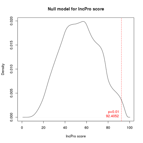
To improve specificity, we further derived the statistical significance of interaction scores reported by lncPro based on empirical NULL distribution generated by random sequence shuffling (see figures below). Interactions with p value <= 0.01 are considered to be significant. To make the results more intuitive, Ensembl IDs are finally converted into HGNC gene symbols. If multiple Ensembl IDs are mapped to one gene symbol, the score with the smallest p value will be reported.

Association studies like Genome-Wide Association Study (GWAS) and expression Quantitative Trait Loc (eQTL) offer unique opportunities to characterize lncRNAs associated with diseases and other traits. In addition to annotating the inputted lncRNA with variants from NHGRI GWAS Catalog, AnnoLnc2 also integrates human multi-tissue eQTLs data from GTEx (pvalue_RE2 < 0.05) and mouse phenotypic and QTL alleles from MGI (length < 10000bp). When reporting human GWAS SNPs, all SNPs linked with the tag SNP (linkage score > 0.5, linkage disequilibrium scores were downloaded from here, tag SNP is linked with itself in all population with score equals to 1) are reported, along with their relative position to the aligned lncRNA (e.g., ‘promoter’, ‘exon’, or ‘intron’) and all relevant information of the tag SNP (i.e., the associated trait, the p-value, the PubMed ID of the paper reporting this SNP). When reporting mouse alleles, the allele’s type, ID, symbol and name, its associated marker’s ID and name as well as the PubMed ID of the paper reporting this allele are listed.

Selection is a direct indicator for biological functions. To effectively identify selection signals across various evolutionary clades, we re-implemented the UCSC MultiZ-Phast pipeline and recomputed conservation scores for primates, mammals and vertebrates clades, following the guide of UCSC. Briefly, we downloaded the 100-way multiple alignments data (hg38) from UCSC Genome Browser, constructed phylogeny for each clade with phyloFit, and computed phastCons score and phyloP score by phast and phyloP, respectively. In addition, AnnoLnc2 also integrates the derived allele frequency (DAF) (1000 Genomes Project Consortium, et al., 2010) of the YRI population (Yoruba in Ibadan, Nigeria) from here for every position (if has corresponding score, and converted from hg19 to hg38 by liftOver) of both the exon and promoter region (upstream 1Kb). For mouse, the 60-way phastCons score and phyloP score of mm10 across Glire, Euarchontoglire, Placental, Vetebrate were directly downloaded from UCSC. To give an overall view, we also calculate the mean conservation scores for exon and promoter regions and finally present them in well-organized bar charts.